|
Important warning : for an efficient fitting of a
2D spectrum, restrict the sizes in both dimensions to a minimum value (see
example spectrum for examples).
Step 1 : calibrate the indirect dimension of the
MQMAS experiment...
 Load the 2D
experiment (2rr file of XWinNMR or 'xxx.rr' file of WinNMR) Load the 2D
experiment (2rr file of XWinNMR or 'xxx.rr' file of WinNMR)
 call the
Spectrum Parameter Dialog [Menu/File/Show Parameters] or click the "Spec Param"
buttion on the left pannel. call the
Spectrum Parameter Dialog [Menu/File/Show Parameters] or click the "Spec Param"
buttion on the left pannel.
 In the
"F2 param" tab select the nucleus of the MQ experiment "27Al" for example. In the
"F2 param" tab select the nucleus of the MQ experiment "27Al" for example.
 Click "F1
param" and "F2 param" tabs (there is a bug in the updating routine) to make the
"Calibrate MQ..." button visible Click "F1
param" and "F2 param" tabs (there is a bug in the updating routine) to make the
"Calibrate MQ..." button visible
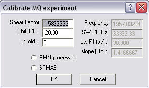
 Click the
"Calibrate MQ..." button which should show this window. Click the
"Calibrate MQ..." button which should show this window.

 The shear
factor is computed for a 3Q experiment and the shift (as used in Bruker shearing
routine) should show in the shift F1 place. If not correct, adjust values. The
nFold value allows you to scroll the F1 dimension. Click the Ok button to
process. The shear
factor is computed for a 3Q experiment and the shift (as used in Bruker shearing
routine) should show in the shift F1 place. If not correct, adjust values. The
nFold value allows you to scroll the F1 dimension. Click the Ok button to
process.
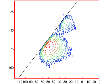
 Once
calibrated you can show the diagonal (slope 1 in ppm) by going to [Menu/2D/DiagSlope]
and setting the slope to 1 (if not already done) The spectrum should show as
presented below. Once
calibrated you can show the diagonal (slope 1 in ppm) by going to [Menu/2D/DiagSlope]
and setting the slope to 1 (if not already done) The spectrum should show as
presented below.

 A good
practice is now to save the calibrated spectrum : [Menu/File/SaveAs] "mycalibratedspectrum.rr"...
Do nor forget the ".rr" extension. A good
practice is now to save the calibrated spectrum : [Menu/File/SaveAs] "mycalibratedspectrum.rr"...
Do nor forget the ".rr" extension.
Step 2 : Establish the fitting model... The better
way is to do that from the fit of a 1D spectrum (see
first how to fit a 1D spectrum and details on the Czsimple model )
 Load the 2D
calibrated spectrum "mycalibratedspectrum.rr" that we just saved, go to
[Menu/2D/Diagonal] and set a slope of 1 to obtain the 1/1 ppm diagonal. Load the 2D
calibrated spectrum "mycalibratedspectrum.rr" that we just saved, go to
[Menu/2D/Diagonal] and set a slope of 1 to obtain the 1/1 ppm diagonal.
 Load the 1D
fit parameters [Menu/Decomposition/load Other] Load the 1D
fit parameters [Menu/Decomposition/load Other]

 Remove from
the fit parameters dialog [Menu/Decomposition/Fit Parameters] or Remove from
the fit parameters dialog [Menu/Decomposition/Fit Parameters] or
 all
lines corresponding to the outer transition only keeping the lines of the
central <1/2> transition "CzSimple" model (if you take my example file, also
remove the smallest AlO6 component which dos not show up in the MQMAS spectrum). all
lines corresponding to the outer transition only keeping the lines of the
central <1/2> transition "CzSimple" model (if you take my example file, also
remove the smallest AlO6 component which dos not show up in the MQMAS spectrum).
 Expand the
window to show the "Fit 1D" selection box at the bottom of the left pannel and
change it to "MQMAS" Expand the
window to show the "Fit 1D" selection box at the bottom of the left pannel and
change it to "MQMAS"
 Click the "Compute
Button" [1234] to obtain the starting Model. This computation takes quite a
while !!! Click the "Compute
Button" [1234] to obtain the starting Model. This computation takes quite a
while !!!
Important remarks
+ Because we now have an F1 axis we need to put a width in this dimension.
This width has to be big enough to obtain a smooth model but not so big as to
mask the expression of the NMR parameters. This "Width" is given in Hertz and
should not be optimized.
+ As in the case of the 1D fit the EM serves to obtain a smoothed
representation of the lineshapes and the distribution of isotropic CS is
obtained with the "FWHM CS" value.
+ As in the case of the 1D fit the d parameter is better fixed to 5 to have a
Gaussian Isotropic Model distribution.
+ Now the computation is long, this is normal as it has to compute for every
point in the 2D spectrum.... Reducing the presentation widow results in quicker
computation and optimisation !!!
+ As in the case of 1D fit with CZSimple, a proper integration is obtained in
the [Report] dialog
 by numerical
integration... Be patient this is a very time consuming operation. by numerical
integration... Be patient this is a very time consuming operation.
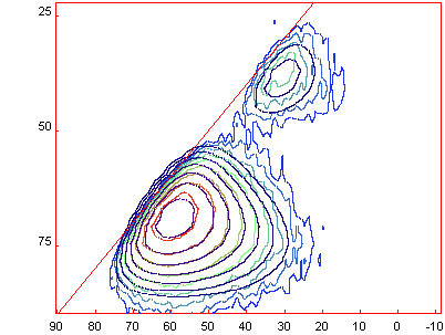
 [Menu/Decomposition/Load
Fit] allows you to laod in the final fit (with 2 Czsimple lines) that give the
following graph : [Menu/Decomposition/Load
Fit] allows you to laod in the final fit (with 2 Czsimple lines) that give the
following graph :

Good luck and be patient with 2D experiments, the more
power you have for computing, the quicker the process...
|
The "CZSimple" Model :
The "CzSimple" model implements a rapid version of the Czjzek
distribution of quadrupolar interaction for the distribution of the isotropic
chemical shift (Gaussian Isotropic Model for d=5) with an uncoupled distribution
of isotropic chemical shift. See our paper in
Geochimica Acta or the
following references for use of this model.
The CzSimple model takes the following parameters :
 Amplitude
: vertical scaling factor Amplitude
: vertical scaling factor
 Position
: Istotropic average value Position
: Istotropic average value
 FWHM
CS : Full Width at Half Maximum of the isotropic chemical shift gaussian
distribution. FWHM
CS : Full Width at Half Maximum of the isotropic chemical shift gaussian
distribution.
 EM au
: line broadening used to smooth the discontinuities issued from the sampling of
nuQ/etaQ and diso, use she smallest possible value and do not allow
optimisation. Take negative values for gaussian apodisation. This is just a
cosmetic parameter. EM au
: line broadening used to smooth the discontinuities issued from the sampling of
nuQ/etaQ and diso, use she smallest possible value and do not allow
optimisation. Take negative values for gaussian apodisation. This is just a
cosmetic parameter.
 nuQ
: Peak value of the quadrupolar coupling of the Czjzek/GIM distribution
(proportional to sigma values reported latest versions >2008) nuQ
: Peak value of the quadrupolar coupling of the Czjzek/GIM distribution
(proportional to sigma values reported latest versions >2008)
 d
: critical exponent of the Czjzek distribution, take d=5 for GIM, other values
do not have physical sense even if they give better rendering. d
: critical exponent of the Czjzek distribution, take d=5 for GIM, other values
do not have physical sense even if they give better rendering.
|